Computer Science Circles: 10 years + 2 million problems

The longest-running project I’ve ever been involved with just turned 10! Computer Science Circles (https://cscircles.cemc.uwaterloo.ca) is a website that teaches introductory programming via Python. It has automatically-graded programming exercises, and in addition, students and teachers can register together, using the site as a place to ask/answer questions and track progress.

The ruminations and brainstorming for the website began in 2009. The name is similar to Math Circles, though Troy also justified it thusly:

I imagined the circles perhaps overlapping in some Venn-like way: doing this module in language X leads to a similar language in language Y. Or maybe they are even touching at various points: go around the Python Circle, and it connects at other points.

Whatever curvature we obtained, the project worked pretty well. At the time of writing, 1,993,555 problems have been solved on the site, with the most popular problem solved by 58,298 registered accounts. (And 1601 accounts have solved the hardest problem.)

We finally decided to ditch our original webserver this year. To that end, I thought some comparisons would be apt:

2010-2011 2019
What happened: Site launched! (First users Sept 2011) New server!
The WordPress: 2.9.2 “Carmen McRae” (Installed May 20, 2010) 5.3 “Rahsaan Roland Kirk”
The hot newness: Python 3 WordPress upgrades with a button click
The crufty oldness: Python 2 Role Scoper, a plugin last updated 3 years ago that I had to delete
OS CentOS 5.x (too obsolete for recent PHP) Ubuntu 18.04
Localizations English, French, … …, German, Dutch, Chinese, Lithuanian

Troy, Sandy and I still answer questions from students on the site. It definitely has been helpful to split the load three ways, but the number of questions was never aggressively overwhelming. There are multiple places online where answers are posted and I wonder to what extent that contributed 🙂

Probably the hardest single maintenance issue over time was when we wanted to add HTTPS to the old server. The awesome letsencrypt.org project gave us a way to do it—sort of—hacking around the incompatibly old PHP version to somehow run the acme certbot. Anyway. The overall construction and maintenance of everything added up to about 2k commits in total on github.

In addition to a paper and a couple of posters on the site itself, the most interesting outcomes to me have been:

  • visiting a jail in Penetanguishene where they cloned the open-source version to teach this without internet access
  • a 2015 paper on frequency distributions of programming errors, using the CS Circles submissions corpus
  • a 2016 paper with educators at a Serbian university on extensions they added to their fork of the site

What do I hope to accomplish in the next 10 years of Computer Science Circles?

  • I’ve been using git subrepositories for ten years, and I still have no idea how they work and how to properly maintain them… that seems like worth learning since I’ve broken things more than once as a result.
  • New content: maybe idiomatic Python data structures such as dictionaries?
  • More localizations. We’ve had multiple false starts on different languages and it would be nice to get another big one out the door (e.g. Spanish).

Last but not least I owe a debt to all the free software on which the site was built, including Linux, Python, WordPress, CodeMirrorPolylang, and FlexiGrid; Mooshak, which we built our safeexec from; and Philip Guo and Peter Wentworth who built the original visualizer and its Python 3 port.

What Is ASCII?

Disclaimer: I am not a historian. I am just a Computer Science educator who likes reading Wikipedia and printing funny characters. This explanation is a long optional appendix for a programming assignment in my course.

ASCII is the American Standard Code for Information Interchange. Developed starting in 1960, it was a way of standardizing means of communication between computers.

To explain, it’s useful to note that “8 bits” means two things from the perspective of a C++ programmer.

  • These days all computers have standardized on organizing memory in bytes. That is to say, each memory address contains 8 bits.
  • In C++, a char variable, representing a single character for communication, is also 8 bits wide.

Neither of these has been true forever. (Actually, some of the earliest computers did not use binary! But we’ll only be talking about bit-based computers here.)

  • There were machines where each memory address contained some other number of bits like 22, 12, 18, 25, etc; see this table on Wikipedia.
  • People used 5-bit Baudot codes for early communication. At 32 possible codes, that was just big enough for the English alphabet, but not lowercase letters or digits. This gradually expanded over the years to 6-bit, 7-bit and finally 8-bit codes.

However, 7 bits was sort of a sweet spot. At 128 possible codes, there was enough room for both lower-case and upper-case letters, digits, punctuation, with space left over for “control codes.” The development of ASCII in the 1960s was led by the American Standards Association. It proposed a standard meaning for all 128 values in a 7-bit code:

  • The first 32 codes (0-31) were specific “control characters.” They didn’t have a direct graphical representation but instead had a specific semantic meaning. Notable examples are #0 the null character, #8 backspace, #9 tab, #10 line feed, and #13 carriage return.
  • Character 32 was a space.
  • Characters 33-126 meant the following, in order:
    #33-63: !"#$%&'()*+,-./0123456789:;<=>
    #64-95: @ABCDEFGHIJKLMNOPQRSTUVWXYZ[\]^_
    #96-126: `abcdefghijklmnopqrstuvwxyz{|}~
  • Character 127 meant “delete”. Here is a quote from Wikipedia that gives a nice explanation:

    This code was originally used to mark deleted characters on punched tape, since any character could be changed to all ones by punching holes everywhere. If a character was punched erroneously, punching out all seven bits caused this position to be ignored (or deleted).

Anyway, the idea of proposing ASCII as a way of standardizing was pretty good. It meant that if you had two machines communicating with each other, they had a chance to understand one another.

ASCII is ubiquitous now, but that was not always the case. Quoting this CNN article,

[T]here was an 18-year gap between the completion of ASCII in 1963 and its common acceptance. … Until 1981, when IBM finally used ASCII in its first PC, the only ASCII computer was the Univac 1050, released in 1964 (although Teletype immediately made all of its new typewriter-like machines work in ASCII).

The most well-known system not compatible with ASCII was EBCDIC. EBCDIC was developed in 1963. It is deeply weird in the sense that the letters of the alphabet don’t all contiguous codes. But there’s reason for this; it has to do with the Hollerith card code. Hollerith worked for the US Census and founded a startup in 1896 that was the precursor to IBM. The common punchcard standard that eventually dominated had 12 rows but not all 2048 combinations were viable, since it would destroy the card’s physical strength. So typical characters in a Hollerith code would punch up to 1 out of three “zone” rows plus up to 1 of out of nine “numeric” rows. Encode this as decimal and you get 36 choices from “00” to “39”. Then encode that as binary and all of a sudden you have a gap, e.g. formerly-adjacent codes 19 and 20 are all of a sudden 011001 and 100000. (This oversimplifies a bit, but a summary of the main point is that the BCD in EBCDIC means binary-coded decimal.)

029-64-250Also, EBCDIC did not contain all the punctuation characters that ASCII did. Some keyboards set up for EBCDIC did not have keys for characters like ^, { or }. See the 1972 international standard ISO 646, which is sort of a missing link between EBCDIC and ASCII. The presence of hardware and operating systems unable to support all characters is the reason that “C digraphs” and “C trigraphs” exist, e.g. that int x = 3 ??' 5 sets x equal to 4. (For applications of C di/trigraphs, see the IOCCC.)

So in a nutshell EBCDIC existed due to the fact that hardware and software’s evolution was gradual and intertwined.

There’s another acronym that you’ll see a lot in researching this subject. Specifically, you’ll sometimes see ANSI as a synonym for ASCII, or to mean a variety of related concepts. What actually happened is that the American Standards Institute, which was the organization to develop ASCII, renamed itself the American National Standards Institute (ANSI) in 1969. From this ASCII gained another name retroactively, the “ANSI X3.4” standard. (And ANSI released more standards later on.)

Towards 8 bits

Eventually, ASCII was adopted more and more, which is why you don’t have an EBCDIC table in the appendix of your textbook. To this day, the word ASCII still technically refers to the 128-character 7-bit system mentioned above.

Over time, computer architectures did eventually standardize on word sizes and addressable locations that used bytes (8 bits). The PDP-8, sold commercially between 1963 and 1979, was the last popular machine whose word size was not a power of 2 (it used 12-bit words).

Hence, there was some wiggle room. A file on your hard drive, or a character being transmitted from computer to computer, or a char variable, actually had 8 bits of space, but ASCII only used 7. If you were to use all 8 bits, you could encode 256 possibilities, which was an extra 128 characters! This was particularly useful for non-English speakers, since most languages use accents or different letters not present in English. Spanish users would be interested in having ñ get one of those values in the unused space from #128-255, while French and Turkish speakers could use ç, Germans would like to add ß, Russians could use И, etc. But, there wasn’t enough space to satisfy everyone.

Enter the code page. This system, which became particularly common with DOS 3.3 in 1987, meant that every user could make their own choice about what system of letters would appear in those extra 128 slots. The most common English code page, CP 437, used those slots for the following characters:

#128-159: ÇüéâäàåçêëèïîìÄÅÉæÆôöòûùÿÖÜ¢£¥₧ƒ
#160-191: áíóúñѪº¿⌐¬½¼¡«»░▒▓│┤╡╢╖╕╣║╗╝╜╛┐
#192-223: └┴┬├─┼╞╟╚╔╩╦╠═╬╧╨╤╥╙╘╒╓╫╪┘┌█▄▌▐▀
#224-254: αßΓπΣσµτΦΘΩδ∞φε∩≡±≥≤⌠⌡÷≈°∙·√ⁿ²■

(The last character #255 is “non-breaking space,” another control character.)

Those lines and boxes were extremely useful in creating an entirely new domain, ASCII art. (Or maybe it is called ANSI art? Technically it should be called CP-437 Art but that name didn’t seem to take off.)

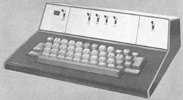
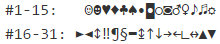
Of special mention is that on many machines of the DOS era, you could directly manipulate the screen’s contents. A program could set your monitor to text mode, for example 80×25 where there are 25 rows and 80 columns, each with room for a single letter. (Your VM looks like this when  it boots up.) This is extremely similar to a bitmap: a 80-by-25 array of char values. In fact, the system assigned visual symbols or glyphs for all possible values from 0 to 255, even the non-printable control codes. So text-based games/art/applications of the day also had access to these symbols (in CP 437):

32

There were many other code pages. Almost all of them stuck to ASCII for the first 128 values (#0-127) and then added the 128 additional characters of local interest. E.g. here is what CP 866 contains at these positions:

#128-159: А‌Б‌В‌Г‌Д‌Е‌Ж‌З‌И‌Й‌К‌Л‌М‌Н‌О‌П‌Р‌С‌Т‌У‌Ф‌Х‌Ц‌Ч‌Ш‌Щ‌Ъ‌Ы‌Ь‌Э‌Ю‌Я
#160-191: а‌б‌в‌г‌д‌е‌ж‌з‌и‌й‌к‌л‌м‌н‌о‌п‌░‌▒‌▓‌│‌┤‌╡‌╢‌╖‌╕‌╣‌║‌╗‌╝‌╜‌╛‌┐
#192-223: └‌┴‌┬‌├‌─‌┼‌╞‌╟‌╚‌╔‌╩‌╦‌╠‌═‌╬‌╧‌╨‌╤‌╥‌╙‌╘‌╒‌╓‌╫‌╪‌┘‌┌‌█‌▄‌▌‌▐‌▀
#224-255: р‌с‌т‌у‌ф‌х‌ц‌ч‌ш‌щ‌ъ‌ы‌ь‌э‌ю‌я‌Ё‌ё‌Є‌є‌Ї‌ї‌Ў‌ў‌°‌∙‌·‌√‌№‌¤‌■‌

The picture is further complicated by right-left languages and joined-letter scripts like Arabic, and languages like traditional Chinese with way more than 128 writing symbols.

In English communication, the Windows-1252 codepage became dominant. Compared to CP 437, it lost the line art, but gained smart quotes, fancy dashes, and other useful punctuation. (This made since because in Windows, they had real windows made out of pixels, rather than line art text mode graphics.)

For our Caesar Decipher assignment, the files will be given to you in the Windows-1252 format. (Technically, the internationally standardized Latin-1 subset.) But it shouldn’t matter, since your program will only do anything to those char values between ‘A’ and ‘z’, which are in the “official” ASCII range between 0 and 127.

Unicode

Most modern communications today, especially international ones, use a more recent system called Unicode.

One problem with the codepage system above is that you don’t really know what a file is saying just by looking at its bits. You can’t be sure if (char)161 means б‌, í, or something else. And there’s absolutely no way to represent a file that contains more than 256 distinct characters. (Such as this very article.)

This was eventually solved by Unicode, which began as an attempt to bring all of the code pages into a single system. Unicode is based on two principles:

  • One unified and fixed numbering of all possible symbols. For example, б is 1073 (“CYRILLIC SMALL LETTER BE”) and í is 237 (“LATIN SMALL LETTER I WITH ACUTE”). Each possible symbol is called a unicode code point.
  • A variety of different encodings, i.e. systems to encode a given sequence of code points as a series of bytes. (The most common encoding these days is UTF-8, a variable-width encoding.)

This system still had its growing pains and we’ll just mention the most noteworthy miscalculation. Joe Becker said in 1988,

Unicode aims in the first instance at the characters published in modern text (e.g. in the union of all newspapers and magazines printed in the world in 1988), whose number is undoubtedly far below 2^14 = 16,384. Beyond those modern-use characters, all others may be defined to be obsolete or rare; these are better candidates for private-use registration than for congesting the public list of generally useful Unicodes.

The Java language was even designed based on this assumption: a Java char is a 16-bit variable. However, this didn’t last long, and as of writing, the latest version of Unicode, version 7.0, contains 113,021 different characters (code points). In Java, this entailed the use of the UTF-16 encoding. In C++, you can read about the platform-dependent wchar type.

For historical context, you might read Kiss your ASCII Goodbye, written in 1992.

One thing is clear: at some point, maybe related to surpassing the 16,384-character limit, the Unicode consortium changed their definition of the “modern-use characters” that could fit in the standard. For example, character 9731 is ☃ (SNOWMAN). Try copying

http://☃.net

into your browser address bar.

Graphs and Bananas

Some fantastic things as of late. (Not more fantastic than previously but still not bad.)

  • A puzzle. You have an integer array of length N in memory, indexed from 1 to N. Each of the integers that it contains is between 1 and N-1. By the pigeonhole principle, two entries are the same. If the array is write-only read-only, can you find two identical entries of the array in O(N) time, using O(log N) additional bits of read-write memory? Thanks to Dan Armendariz for telling me about this at SIGCSE.
  • A game. Binary tree isomorphism? There’s an app for that. The game Splice is based on this at some level, where you have a limited number of moves to adjust one tree to make it into another. This is alone a nice kind of puzzle, especially since it’s NP-complete. But what is the most striking about this game is its beautiful user interface. Very responsive and fluid, behaves well with a touchscreen. Excellently themed. Getting started is rough since the instructions are tucked away in a corner. Probably my favourite Android game, although I have not found that many contenders.
  • A book. Ij9531n Pursuit of The Travelling Salesman by Bill Cook describes a classical problem in computer science and mathematics in a way that is both scientifically elegant and humanistically down-to-earth. This is probably my favourite book out of anything I could hand to an undergrad and get them to care about the P vs NP problem. The writing explains insights without being technical, and presents interesting stories about the researchers without turning into biographies.
  • A movie. There is also a movie Travelling Salesman, which recently completed an IndieGogo campaign, dealing with the same problem. According to Bill Cook, the film almost had to cancel production in the middle of 2010 when an alleged proof of P != NP was circulated. (Although, aren’t a lot of good fictional movies based on false premises?) Perhaps my favourite thing about this movie is that the main character shares a name with a beloved Canadian hockey player-cum-coffee mascot.
  • Muffins. Not sure why I like bananas only when they are a component in a baked good, but there you go.

A Boole’s Errand

Did you know this is the last day of CS Education Week? The creators of this event are highly engaged in bringing Computer Science to more high schools — in many states, CS is not given full consideration in the curriculum and this is shocking to me given that children are using computers not much later than they can read and write. But, let me leave you with a link to a very detailed report if you want to know more, and instead ask you some puzzles.

In Boolean algebra (named after George Boole) you manipulate the symbols T (for true) and F (for false). This is useful to help analyze, understand, and simplify the flow of logic in computer programs and electronic circuits. The NOT function swaps T to F and vice-versa, for example NOT(F) = T and NOT(T) = F. One way to combine two values is with the OR function: if you give it two of the same input it gives you the same one back, but if you give it a mix of T’s and F’s it gives you back T. For example OR(T, F) = T and OR(F, F) = F. AND does the same thing, but it gives you back F if the inputs are a mix of T and F.

A couple of miraculous things happen from these definitions. One is DeMorgan‘s Law, which says that

  • NOT(AND(x, y)) = OR(NOT(x), NOT(y)), no matter what the values of x and y are;
  • similarly NOT(OR(xy)) = AND(NOT(x), NOT(y)).

In a sense, this law says that NOT turns AND in to OR and vice-versa.

Another one is that we get a distributive law

  • AND(x, OR(y, z)) = OR(AND(x, y), AND(x, z)), no matter what the values of x, y, and z are;
  • similarly OR(x, AND(y, z)) = AND(OR(x, y), OR(x, z)).

So this is like arithmetic where x*(y+z) = x*y + x*z but continuing the analogy, somehow for Boolean algebra we also have x+y*z = (x+y)*(x+z), which is not like arithmetic.

Finally, there is a function XOR (exclusive or) which is a cousin of OR. Note that in English sometimes we use “or” to mean the “OR” function described  above: “you’re not allowed to drive if you have no license OR you’re drunk” (or both). But in English sometimes “or” means “either but not both,” like “this combo comes with a salad or fries” — in this case you can’t get both. This is XOR in Boolean logic: it has the same behaviour as OR except that XOR(T, T)=F instead of how OR(T, T) = T. It turns out that there are a couple of ways to build XOR,

  • AND(OR(x, y), OR(NOT(x), NOT(y))) is one definition of XOR(x, y)
  • OR(AND(x, NOT(y)), AND(NOT(x), y)) is another equivalent definition of XOR(x, y).

I’d call this equivalence another law.

Here are some questions:

  1. Troolean logic. Let’s say we extend Boolean logic to have a third value ? meaning “I don’t know.” So we should define NOT(?)=?, as well as OR(F, ?) = ? and OR(T, ?) = T since in the first case we can’t tell what the result of OR should be, but in the second it should definitely return T. Show that we can define AND and XOR on all pairs of inputs involving T, F, and ? so that all of the laws above hold.
  2. Quadroolean logic. Instead, we could extend Boolean logic to have 4 values: F, T, VF and VT, where VF is “very false” and VT is “very true.” Thus NOT(VF)=VT and NOT(VT)=VF makes a sensical definition, as well as OR(VF, x) = x for all x and OR(VT, x) = VT for all x. Show that we can define AND and XOR on all pairs of inputs involving T, F, VT and VF so that all of the laws above hold.
  3. n-oolean logic. Show that for any integer n > 1, we can come up with a set of exactly n symbols including T and F, and definitions of NOT, AND, OR and XOR for them so that all of the laws above hold, plus a few others: NOT(NOT(x)) = x; the commutative property AND(x, y)=AND(y, x) and similarly for OR; the associative property AND(x, AND(y, z)) = AND(AND(x, y), z) and similarly for OR; the idempotent laws OR(x, x) = AND(x, x) = x.
  4. Are there multiple truly different n-oolean logics?
  5. Does the XOR equivalence law follow automatically from all of the other laws? (This one I don’t know the answer to.)

Virtual Valuations

Last weekend I attended a conference in Budapest where I saw a nice trick in an unexpected place. (A longer report about the whole trip will appear on the CS Theory Blog.) Wikipedia calls it de Moivre’s martingale and the reason that I liked it is that it somehow gives me some intuition, that I formerly lacked, about virtual valuations in Myerson’s seminal result about obtaining profit-maximizing auctions from welfare-maximizing auctions.

To give some background to de Moivre’s martingale, consider the following problem: take a fair random walk in which you walk left or right by 1 unit in each step with probability 1/2; calculate the expected squared distance from the origin after n steps. One method is to explicitly calculate the value using some binomial coefficients, and do painful simplications, giving the answer n. But there is a simpler method to get this simple answer: notice that, conditioned on your position p(t) at time t, the expected increase in square distance at time t+1 is

E[p^2(t+1)-p^2(t)|p^2(t)] = 1/2(p(t)+1)^2+1/2(p(t)-1)^2-p^2(t) = 1.

So unconditioning and using linearity of expectation, we get E[p(n)^2] = 1 + 1 + ... + 1 + 0 = n.

de Moivre’s martingale

Suppose you are participating in a biased random walk where on each step you move left with probability L≠1/2 and right with probability R=1-L. You can think of this as gambling. Say you start at position x, representing that you have $x. Now let’s play until either you run out of money (hit position 0) or you break the bank (hit position y>x). What is the probability of each of these two cases (win/lose), as a function of L, x, y?

Again, a direct calculation seems possible but is nasty. But instead, we can define a virtual position. We will define a function f : Nand when the real position at time t is p(t), the virtual position at time t is f(p(t)). In fact, we will define the virtual positions so that the martingale formula holds:

E[f(p(t+1))|p(t)] = f(p(t)).

This would mean that f(p(t)) is a martingale in t, that is to say, its expected value is the same in each time step. If we can accomplish this, then by comparing the final virtual position to the initial one, we deduce a formula for what we want (end is the stopping time, a random variable):

f(x) = f(p(0)) = E[f(p(end))] = Pr[win]*f(y) + Pr[lose]*f(0)

so

Pr[win] = (f(x)-f(0))/(f(y)-f(0)).

If you think about the martingale formula for a few minutes, you find that f satisfies a second-order linear recurrence relation, L*f(m-1)+R*f(m+1) = f(m). Standard methods give all the solutions of this recurrence, almost any will do, but the simplest is to take f(m) = (L/R)^m. Then the probability of winning is ((L/R)^x - 1)/((L/R)^y - 1)!

Myerson

What Myerson accomplished is to show basically that the celebrated “VCG mechanism” for combinatorial auctions, which is truthful and maximizes social welfare, can be converted into a truthful mechanism to maximize the auctioneer’s income, under mild technical assumptions, in the model that bidder’s distributions on valuations are known in advance. Myerson’s method is to replace each valuation with a “virtual valuation” that looks mysterious at first, but is similar to the above example, in the sense that you define the function based on the properties that you want it to have.  My lecture notes from last term explain this in a more precise way. I am glad now to have this valuable intuition!

Depth and Violation

Over the last year or so I became interested in a family of problems related to linear programming. In ordinary linear programming, we are given some collection of linear constraints, say {ai x ≥ bi} for i=1, …, n, and the x represents a d-dimensional variable. A central result in optimization says that there is an efficient algorithm to determine whether any x exists which simultaneously satisfies all of the constraints. However, if not (i.e. if the program is not feasible), it is interesting to ask: what is the maximum number of constraints that we can satisfy? Or equivalently, what is the minimum number of constraints that need to be deleted, in order for the program to become feasible?

A half-plane

Caveat: these are rough notes, mostly written up for my own benefit, so they may have some bugs, reader beware! (Note to future self: this includes you.)

It is natural to view the problem in a geometric way: each {x | ai x ≥ bi} is a half-space and we are seeking a point which lies in the maximum number of the half-spaces. In geometry you often call the number of half-spaces containing a given x the depth of x so we are equivalently looking for a point x of maximum depth. However, the complementary sets {x | ai x < bi} are open half-spaces so this is the same problem as looking for a point of minimum depth (glossing over the difference between openness and closedness).

In any fixed dimension, these sort of problems can be solved exactly in polynomial time, but they become NP-complete if the dimension is part of the input. Moreover, the approximability of the minimization and maximization versions become different. Below, I sum up what is known for the different versions. Moreover, I also consider the closely related problem of equality systems where each equation looks like {ai x = bi}; in this case geometrically the half-spaces are replaced by hyperplanes.

Maximum halfspace depth. There is no n1-ε approximation [Feige and Reichman], but there is a n/log n approximation by Halldórsson.

Minimum halfspace depth. There is no 2log^(1-ε) n approximation [Arora et al]. There seems to be no nontrivial approximation known in terms of n; but a (d+1)-approximation can be obtained using Helly’s Theorem applied to halfspaces. (There is an algorithm with time polynomial in n and OPTd, e.g. this is poly-time when d = log n and OPT is constant.)

Maximum hyperplane depth. There is no PTAS, but there is a 2-approximation. [Amaldi annd Kann]

Minimum hyperplane depth. Trivially, the answer is 0.

Minimum depth, ≠ constraints (same as minimum deletion to make equality system feasible, or “min unsatisfy”). There is no 2log^(1-ε) n approximation [Arora et al] but there is an εn/log n approximation [Berman and Karpinski].

Maximum depth, ≠ constraints. Trivial again.

You could consider weighted versions where you there is a certain dollar value for satisfying/deleting a given constraint, with the original problems corresponding to all values equalling 1. I would say that “typically” such problems resemble the original versions if all the weights are nonnegative. However, what is the complexity of minimum hyperplane depth if you have weights that are a mix of positive and negative numbers?

In the negative feedback arc set problem, we are given a directed graph with positive and negative arc lengths, and want to delete a minimum-size subset of arcs to destroy all negative-weight cycles. This can be reduced to maximum halfspace depth by using node potentials. Negative feedback arc set automatically inherits constant inapproximability; I don’t think anything else is known about this interesting problem.

FYI: The utility of the Arora et al. paper was observed by Amaldi and Kann in papers from 1995 and1998, which are useful references, although now dated. A recent paper of Gottlieb and Neylon that connects min unsatisfy to other matrix sparsity problems gives 2log^(1/2-ε) n as the resulting hardness but I haven’t checked which is right. The recent paper of Elbassioni et al. has useful references too.

Saarbrücken

Last weekend I went to a two-day workshop on combinatorics at the Max Planck Institut für Informatik. The place is sort of a European mecca for computer science, as it hosts a gigantic collection of post-docs and students, but had only one professor up until recently.

This Guy
Historical Figure

In the city, nearly every restaurant has a logo of this man’s silhouette (see right). Does this indicate the founder of the town? Some historic figure of great repute? Yes, a local told me it is the picture of the founder of the Karlsberg brewery.

There were four invited talks, one of which was by Daniela Kühn. She gave a survey of a remarkable collection of her results with  Deryk Osthus and other co-authors. In brief, there are a whole bunch of open questions about directed graphs from the 1970s, and her results prove that they are true up to any desired tolerance ε, provided the graphs are large enough. The results rely on uses of the “Szemeredi regularity lemma” and the method seems only to work on dense graphs.

Breakfast
Breakfast

As for food, there were tasty things to be had at the Stiefel brewery where the initial get-together was held, but on the last morning I ventured into town to find something even better. The cinnamon pastry shown (which mysteriously had some bites missing by the time I remembered to take a picture of it) came from the Schubert cafe. The Saarlander in my group at EPFL confirms the tastiness of their goods.

Finally, here is a question raised in the talk of Carola Winzen. Alice selects an n-bit binary string x uniformly at random. Then Bob gets to make queries of the form “what is the dot product of x and q” for any binary string q (so the answer is in {0, 1, …, n}) and wants to determine x using as few queries as possible. How many queries does he need (in expectation w.r.t x)? One can easily show a lower bound ~ n/log n, while there is a deterministic upper bound of n. One may show that even if Bob’s queries are totally random, he can uniquely pin down x using ~ n/log n queries. However, the proof doesn’t give Bob an algorithm running in time polynomial(n). Is there an efficient algorithm for Bob using O(n/log n) queries?

Update Yes! The earliest likely candidate is a paper in the Publications of the Mathematical Institute of the Hungarian Academy of Sciences, but I have not tried to dig it up. I did read the slightly later paper “Determination of a subset from certain combinatorial properties” which gives a deterministic poly-time solution, using recursion.